38 display data labels in excel

How to Use Cell Values for Excel Chart Labels - How-To Geek Select the chart, choose the "Chart Elements" option, click the "Data Labels" arrow, and then "More Options." Uncheck the "Value" box and check the "Value From Cells" box. Select cells C2:C6 to use for the data label range and then click the "OK" button. The values from these cells are now used for the chart data labels. How to add data labels from different column in an Excel chart? Right click the data series in the chart, and select Add Data Labels > Add Data Labels from the context menu to add data labels. 2. Click any data label to select all data labels, and then click the specified data label to select it only in the chart. 3.

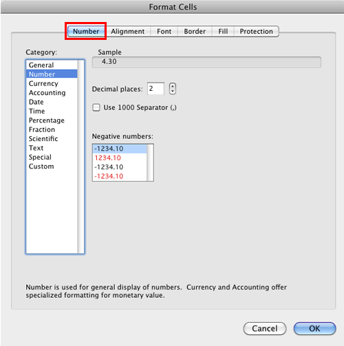
How to show data label in "percentage" instead of - Microsoft Community Select Format Data Labels Select Number in the left column Select Percentage in the popup options In the Format code field set the number of decimal places required and click Add. (Or if the table data in in percentage format then you can select Link to source.) Click OK Regards, OssieMac Report abuse 8 people found this reply helpful ·

Display data labels in excel

Adding rich data labels to charts in Excel 2013 | Microsoft 365 Blog To add a data label in a shape, select the data point of interest, then right-click it to pull up the context menu. Click Add Data Label, then click Add Data Callout . The result is that your data label will appear in a graphical callout. In this case, the category Thr for the particular data label is automatically added to the callout too. Format Data Labels in Excel- Instructions - TeachUcomp, Inc. Then select the "Format Data Labels…" command from the pop-up menu that appears to format data labels in Excel. Using either method then displays the "Format Data Labels" task pane at the right side of the screen. Set the values and positioning of the data labels in the "Label Options" category, which is shown by default. Custom Data Labels with Colors and Symbols in Excel Charts - [How To ... The basic idea behind custom label is to connect each data label to certain cell in the Excel worksheet and so whatever goes in that cell will appear on the chart as data label. So once a data label is connected to a cell, we apply custom number formatting on the cell and the results will show up on chart also.

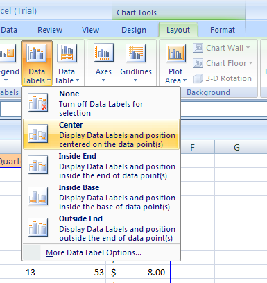
Display data labels in excel. How to Print Labels from Excel - Lifewire Select Mailings > Write & Insert Fields > Update Labels . Once you have the Excel spreadsheet and the Word document set up, you can merge the information and print your labels. Click Finish & Merge in the Finish group on the Mailings tab. Click Edit Individual Documents to preview how your printed labels will appear. Select All > OK . Adding Data Labels to Your Chart (Microsoft Excel) - ExcelTips (ribbon) Click the Data Labels tool. Excel displays a number of options that control where your data labels are positioned. Select the position that best fits where you want your labels to appear. To add data labels in Excel 2013 or later versions, follow these steps: Activate the chart by clicking on it, if necessary. Add data labels and callouts to charts in Excel 365 - EasyTweaks.com Step #3: Format the data labels. Excel also gives you the option of formatting the data labels to suit your desired look if you don't like the default. To make changes to the data labels, right-click within the chart and select the "Format Labels" option. How to format axis labels individually in Excel - SpreadsheetWeb Double-click on the axis you want to format. Double-clicking opens the right panel where you can format your axis. Open the Axis Options section if it isn't active. You can find the number formatting selection under Number section. Select Custom item in the Category list. Type your code into the Format Code box and click Add button.

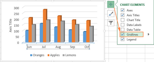
Excel tutorial: How to use data labels Generally, the easiest way to show data labels to use the chart elements menu. When you check the box, you'll see data labels appear in the chart. If you have more than one data series, you can select a series first, then turn on data labels for that series only. You can even select a single bar, and show just one data label. How to Print Address Labels From Excel? (with Examples) - WallStreetMojo First, select the list of addresses in the Excel sheet, including the header. Go to the "Formulas" tab and select "Define Name" under the group "Defined Names.". A dialog box called a new name is opened. Give a name and click on "OK" to close the box. Step 2: Create the mail merge document in the Microsoft word. Data Labels in Excel Pivot Chart (Detailed Analysis) 7 Suitable Examples with Data Labels in Excel Pivot Chart Considering All Factors 1. Adding Data Labels in Pivot Chart 2. Set Cell Values as Data Labels 3. Showing Percentages as Data Labels 4. Changing Appearance of Pivot Chart Labels 5. Changing Background of Data Labels 6. Dynamic Pivot Chart Data Labels with Slicers 7. Add or remove data labels in a chart - support.microsoft.com Right-click the data series or data label to display more data for, and then click Format Data Labels. Click Label Options and under Label Contains, select the Values From Cells checkbox. When the Data Label Range dialog box appears, go back to the spreadsheet and select the range for which you want the cell values to display as data labels.

How To Add Data Labels In Excel - weekir.northminster.info Data labels are used to display source data in a chart directly. Change position of data labels. Source: . The column chart will appear. For example, this is how we can add labels to one of the data series in our excel chart: Source: . Click the + symbol and add data labels by clicking it as shown below step 3 ... Quick Tip: Excel 2013 offers flexible data labels | TechRepublic right-click and choose Insert Data Label Field. In the next dialog, select [Cell] Choose Cell. When Excel displays the source dialog, click the cell that contains the MIN () function, and click OK.... How to Create Labels in Word from an Excel Spreadsheet - Online Tech Tips Select Browse in the pane on the right. Choose a folder to save your spreadsheet in, enter a name for your spreadsheet in the File name field, and select Save at the bottom of the window. Close the Excel window. Your Excel spreadsheet is now ready. 2. Configure Labels in Word. Change the format of data labels in a chart To get there, after adding your data labels, select the data label to format, and then click Chart Elements > Data Labels > More Options. To go to the appropriate area, click one of the four icons ( Fill & Line, Effects, Size & Properties ( Layout & Properties in Outlook or Word), or Label Options) shown here.

Apply Custom Data Labels to Charted Points - Peltier Tech

How to Add Data Labels to an Excel 2010 Chart - dummies On the Chart Tools Layout tab, click Data Labels→More Data Label Options. The Format Data Labels dialog box appears. You can use the options on the Label Options, Number, Fill, Border Color, Border Styles, Shadow, Glow and Soft Edges, 3-D Format, and Alignment tabs to customize the appearance and position of the data labels.

Apply Custom Data Labels to Charted Points - Peltier Tech

Data labels not displayed correctly - Excel Help Forum The data label is a date value that selects values from the date column. The Primary axis is categorized based on 2 values. The secondary axis is Month. The data labels are displayed accurately as per the month except the 3 labels. The first series is the difference between F and E.The second series is the difference between the J and K column.

Excel sunburst chart: Some labels missing - Stack Overflow

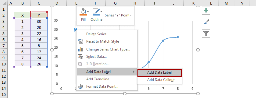
How to add data labels in excel to graph or chart (Step-by-Step) Add data labels to a chart. 1. Select a data series or a graph. After picking the series, click the data point you want to label. 2. Click Add Chart Element Chart Elements button > Data Labels in the upper right corner, close to the chart. 3. Click the arrow and select an option to modify the location. 4.

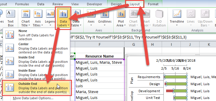
Add Outside End Data Labels to Resource Filler Series - Excel ...

Excel charts: how to move data labels to legend @Matt_Fischer-Daly . You can't do that, but you can show a data table below the chart instead of data labels: Click anywhere on the chart. On the Design tab of the ribbon (under Chart Tools), in the Chart Layouts group, click Add Chart Element > Data Table > With Legend Keys (or No Legend Keys if you prefer)

Adding Data Labels to Your Chart (Microsoft Excel)

How to add text labels on Excel scatter chart axis - Data Cornering Add dummy series to the scatter plot and add data labels. 4. Select recently added labels and press Ctrl + 1 to edit them. Add custom data labels from the column "X axis labels". Use "Values from Cells" like in this other post and remove values related to the actual dummy series. Change the label position below data points.

Add or remove data labels in a chart

Find, label and highlight a certain data point in Excel scatter graph Here's how: Click on the highlighted data point to select it. Click the Chart Elements button. Select the Data Labels box and choose where to position the label. By default, Excel shows one numeric value for the label, y value in our case. To display both x and y values, right-click the label, click Format Data Labels…, select the X Value and ...

How to Add Data Labels in Excel - Excelchat | Excelchat

Custom Chart Data Labels In Excel With Formulas - How To Excel At Excel Follow the steps below to create the custom data labels. Select the chart label you want to change. In the formula-bar hit = (equals), select the cell reference containing your chart label's data. In this case, the first label is in cell E2. Finally, repeat for all your chart laebls.

How to use data labels in a chart

How to Show Percentage in Bar Chart in Excel (3 Handy Methods) - ExcelDemy Likewise, we create a Data Labels (-) column. =IF (D5>C5,E5/D5,"") After completing the above steps the data table should look like the image shown below. 📌 Step 02: Insert Clustered Bar Chart and Add Formatting Secondly, select the dataset and go to Insert > Insert Column or Bar Chart > Clustered Column Chart. The chart appears as shown below.

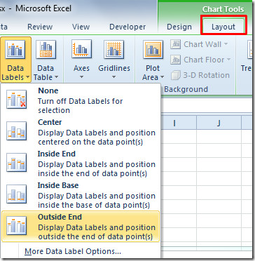
Excel 2010: Show Data Labels In Chart

Show numbers in thousands in Excel as K in table or chart - Data Cornering If you want to show numbers in thousands or millions on the Excel chart axis, change the axis display units options. Format axis (select axis labels, and press Ctrl + 1) and change display units like this. As the result, you will get something like this.

How to insert data labels to a Pie chart in Excel 2013

How to add or move data labels in Excel chart? - ExtendOffice 2. Then click the Chart Elements, and check Data Labels, then you can click the arrow to choose an option about the data labels in the sub menu. See screenshot: In Excel 2010 or 2007. 1. click on the chart to show the Layout tab in the Chart Tools group. See screenshot: 2. Then click Data Labels, and select one type of data labels as you need ...

Fixed:] Excel Chart Is Not Showing All Data Labels (2 Solutions)

Custom Data Labels with Colors and Symbols in Excel Charts - [How To ... The basic idea behind custom label is to connect each data label to certain cell in the Excel worksheet and so whatever goes in that cell will appear on the chart as data label. So once a data label is connected to a cell, we apply custom number formatting on the cell and the results will show up on chart also.

Excel 2013: Charts

Format Data Labels in Excel- Instructions - TeachUcomp, Inc. Then select the "Format Data Labels…" command from the pop-up menu that appears to format data labels in Excel. Using either method then displays the "Format Data Labels" task pane at the right side of the screen. Set the values and positioning of the data labels in the "Label Options" category, which is shown by default.